Students taking this course for 4 credits are requied to do this assignment. Students taking this course for 3 credits may do this assignment if the wish; if so, all parts count as optional points for them.
Reference input and output files are included below; the full set can be downloaded as mprayfiles.zip. Do not upload these files as part of your submission: the grading server will supply them instead.
This assignment, like all other assignments, is governed by the common components of MPs.
1 Overview
This programming assignment created 3D imagery using ray tracing. In most other respects, its logistics are similar to the rasterizer assignment: you code in any language you want and your program reads a text file and produces an image file.
1.1 Ray Emission
Rays will be generated from a point to pass through a grid in the
scene. This corresponds to flat projection,
the same kind that
frustum matrices achieve. Given an image w pixels wide and h pixels high, pixel (x, y)’s ray will be based the following
scalars:
s_x = {{2 x - w} \over {\max(w, h)}}
s_y = {{h - 2 y} \over {\max(w, h)}}
These formulas ensure that s_x and s_y correspond to where on the screen the pixel is: s_x is negative on the left, positive on the right; s_y is negative on the bottom, positive on the top. To turn these into rays we need some additional vectors:
eye- initially (0, 0, 0). A point, and thus not normalized.
forward-
initially (0, 0, -1). A vector, but not
normalized: longer
forwardvectors make for a narrow field of view. right- initially (1, 0, 0). A normalized vector.
up- initially (0, 1, 0). A normalized vector.
The ray for a given (s_x, s_y) has
origin eye and direction forward + s_x right + s_y up.
1.2 Ray Collision
Each ray will might collide with many objects. Each collision can be characterized as o + t \vec{d} for the ray’s origin point o and direction vector \vec{d} and a numeric distance t. Use the closest collision in front of the eye (that is, the collision with the smallest positive t).
Raytracing requires every ray be checked against the full scene of objects. As such your code will proceed in two stages: stage 1 reads the input file and sets up a data structure storing all objects; stage 2 loops over all rays and intersects each with objects in the scene.
Many of the optional parts of this assignment have rays spawn new rays upon collision. As such, most solutions have a function that, given a ray, returns which object it hit (if any) and where that hit occurred (the t value may be enough, but barycentric cordinates may also be useful); that function is called from a separate function that handles lighting, shadows, and so on.
1.3 Illumination
Basic illumination uses Lambert’s law: Sum (object color) times (light color) times (normal dot direction to light) over all lights to find the color of the pixel.
Make all objects two-sided. That is, if the normal points away from the eye (i.e. if \vec d \cdot \vec n > 0), invert it before doing lighting.
Illumination will be in linear space, not sRGB. You’ll need to convert RGB (but not alpha) to sRGB yourself prior to saving the image, using the official sRGB gamma function: L_{\text{sRGB}} = \begin{cases} 12.92 L_{\text{linear}} &\text{if }L_{\text{linear}} \le 0.0031308 \\ 1.055{L_{\text{linear}}}^{1/2.4}-0.055 &\text{if }L_{\text{linear}} > 0.0031308 \end{cases}
2 Required Features
- png width height filename
- same syntax and semantics as in the rasterizer assignment.
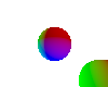
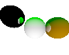
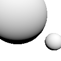
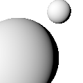
- sphere x y z r
-
 Add a sphere with center (x, y, z) and
radius r to the list of objects to be
rendered. The sphere should use the current color as its color (also the
current shininess, tecture, etc. if you add those optional parts).
Add a sphere with center (x, y, z) and
radius r to the list of objects to be
rendered. The sphere should use the current color as its color (also the
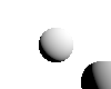
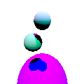
current shininess, tecture, etc. if you add those optional parts).For the required part you only need to be able to draw the outside surface of spheres.
If you see the central sphere but not the one in the corner, the most common reason is failing to normalize ray directions when they are first created. - sun x y z
-
 Add a sun light infinitely far away in the (x,
y, z) direction. That is the
Add a sun light infinitely far away in the (x,
y, z) direction. That is the direction to light
vector in the lighting equation is (x, y, z) no matter where the object is.Use the current color as the color of the sunlight.
For the required part you only need to be able to handle scenes with zero light sources and scenes with one light source.
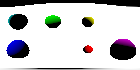
- color r g b
-
 Defines the current color to be r g b,
specified as floating-point values; (0, 0,
0) is black, (1, 1, 1) is white,
(1, 0.5, 0) is orange, etc. You only
need to track one color at a time. If no
Defines the current color to be r g b,
specified as floating-point values; (0, 0,
0) is black, (1, 1, 1) is white,
(1, 0.5, 0) is orange, etc. You only
need to track one color at a time. If no colorhas been seen in the input file, use white.You’ll probably need to map colors to bytes to set the image. First change colors ≤ 0.0 to 0 and colors ≥ 1 to 1; then apply a gamma function; then scale up linearly to the 0–255 byte range. The exact rounding used is not important.
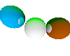
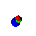
- Overlap
-
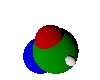
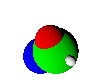 Your rays should hit the closest object even if there are several
overlaping.
Your rays should hit the closest object even if there are several
overlaping.
- sRGB
- Your computations should be in a linear color space, converted to sRGB before saving the image. This is reflected in the colors of every reference image on this page.
- Rays, not lines
-
 Don’t find intersections behind the ray origin.
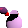
- Shadows
-
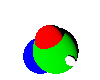
 Spheres should cast shadows on other spheres.
Self-shadowing (sometimes called
shadow acne
) is a problem with many shadow implementations. You should avoid that either with ray origin object IDs (i.e. shadow rays cannot see the sphere that generated them) or collision biases (i.e. shadow rays cannot see objects until they get a millionth of a unit away from their origin).
3 Optional Features (0–220 points)
3.1 Geometry (5–50 points)
- Handle interiors (requires
bulb) (10 points) -
 Correctly render when the camera is inside a sphere
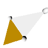
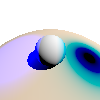
- plane A B C D (5 points)
-
 defines the plane that satisfies the equation Ax + By + Cz + D = 0
It is common to have spurious shadows near the horizon of planes; the reference image shows an example of this just to the left of the sphere. These can be removed with with more careful handling of shadow acne, but doing so is not required for this assignment.
- Triangle (requires plane) (15 points)
-
 Add
Add xyzandtrifcommands, with the same meaning as in the rasterizer assignment (except ray-traced, not rasterized). - Interpolate triangles (requires triangle) (5–20 points)
-
Triangles can have values interpolated in ray tracing using Barycentric coordinates. Examples of values to interpolate:
- normal x y z (5 points)
-
 Defines a normal, which will be attached to all subsequent triangle
vertices and interpolated during scan conversion using barycentric
coordinates.
Defines a normal, which will be attached to all subsequent triangle
vertices and interpolated during scan conversion using barycentric
coordinates.
- trit i_1 i_2 i_3 and texcoord s t (15 points)
-
 The same meaning as in the rasterizer
assignment; see also Textures
The same meaning as in the rasterizer
assignment; see also Textures
3.2 Acceleration (30 points)
Add a spatial bounding hierarchy so that hi-res scenes with thousands of shapes can be rendered in reasonable time.
The basic idea of a bounding hierarchy is simple: have a few large bounding objects, each with pointers to all of the smaller objects they overlap. Only if the ray intersects the bounding object do you need to check any of the objects inside it.
For good performance, you’ll probably need a hierarchy of objects in a tree-like structure. In general, a real object might be pointed to from several bounding objects.
 Because the goal of a spatial bunding hierarchy is speed, we require
both that the code has such a hierarchy in use and that it can render
the scene shown here (which uses two suns and contains 1001 spheres) in
less than a second. And yes, this is arbitrary wall-clock time on our
test server, and yes this does disadvantage people writing in Python
(which is tens to hundreds of times slower than the other languages
people are using in this class).
Because the goal of a spatial bunding hierarchy is speed, we require
both that the code has such a hierarchy in use and that it can render
the scene shown here (which uses two suns and contains 1001 spheres) in
less than a second. And yes, this is arbitrary wall-clock time on our
test server, and yes this does disadvantage people writing in Python
(which is tens to hundreds of times slower than the other languages
people are using in this class).
3.3 Lighting (5–60 points)
- Multiple
suns (5 points) -
 allow an unlimited number of
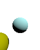
 suncommands; combine all of their contributions; - bulb x y z (requires multiple suns) (10 points)
-
 Add a point light source centered at (x, y,
z). Use the current color as the color of the bulb. Handle as
many
Add a point light source centered at (x, y,
z). Use the current color as the color of the bulb. Handle as
many bulbs andsuns as there are in the scene.Include fall-off to bulb light: the intensity of the light that is d units away from the illuminated point is 1 \over d^2.
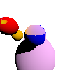
- Negative light (requires
bulb) (5 points) -
 Allow light colors to be less than zero, emitting
 darkness
. - More shadows (5–20 points)
-
 If you add more types of gemetry and lights, shadow casting becomes more
complicated. These points are for handling shadows properly:
If you add more types of gemetry and lights, shadow casting becomes more
complicated. These points are for handling shadows properly:+5 points if planes work, +5 if triangles work, +5 if multiple light sources work, +5 if bulbs work.
Self-shadowing is a problem with many shadow implementations. An occasional spurious shadow near the edge of an infinite plane is fine, but otherwise there should be no extraneous shadows.
- expose v (10 points)
-
 Render the scene with an exposure function, applied prior to gamma
correction. Use a simple exponential exposure function: \ell_{\text{exposed}} = 1 - e^{\displaystyle
-\ell_{\text{linear}} v}.Fancier exposure functions used in industry graphics, such as FiLMiC’s popular Log V2, are based on large look-up tables instead of simple math but are conceptually similar to this function.
Render the scene with an exposure function, applied prior to gamma
correction. Use a simple exponential exposure function: \ell_{\text{exposed}} = 1 - e^{\displaystyle
-\ell_{\text{linear}} v}.Fancier exposure functions used in industry graphics, such as FiLMiC’s popular Log V2, are based on large look-up tables instead of simple math but are conceptually similar to this function. - gi d (requires
aa, andtrif) (20 points) -
 Render the scene with global illumination with depth d. When lighting any point, include as an
additional light the illuminated color of a random ray shot from that
point.
Render the scene with global illumination with depth d. When lighting any point, include as an
additional light the illuminated color of a random ray shot from that
point.These secondary
global illumination
rays should use all of your usual illumination logic to pick their color, including shininess, transparency, roughness, and so on if you’ve implemented them. However, a global illumination ray should only spawn another global illumination ray if d > 1, with the total number of global illumination rays generated capped by d.Distribute the random rays to reflect Lambert’s law. A simple way to do this is to have the ray direction be selected uniformly from inside a sphere centered at the tip of the normal vector with a radius equal to the normal vector’s length.
3.4 Materials (5–65 points)
- shininess s (10 points)
-
 Future objects have a reflectivity of s, which will always be a number between 0
and 1.
Future objects have a reflectivity of s, which will always be a number between 0
and 1.If you implement transparency and shininess, shininess takes precident; that is,
shininess 0.6andtransparency 0.2combine to make an object 0.6 shiny, ((1-0.6) \times 0.2) = 0.08 transparent, and ((1-0.6) \times (1-0.2)) = 0.32 diffuse.Per page 153 of the glsl spec, the reflected ray’s direction is
\vec{I} - 2(\vec{N} \cdot \vec{I})\vec{N}
… where \vec{I} is the incident vector, \vec{N} the unit-length surface normal.
Bounce ech ray a maximum of 4 times unless you also implement
bounces. - shininess s_r s_g s_b (5 points)
-
 Future objects have a different reflectivity for each of the three color
channels.
Future objects have a different reflectivity for each of the three color
channels.
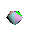
- transparency t (requires
shininess) (15 points) -
 Future objects have a transparency of t, which will always be a number between 0
and 1.
Future objects have a transparency of t, which will always be a number between 0
and 1.Per page 153 of the glsl spec, the refracted ray’s direction is
k = 1.0 - \eta^2 \big(1.0 - (\vec{N} \cdot \vec{I})^2\big) \eta \vec{I} - \big(\eta (\vec{N} \cdot \vec{I}) + \sqrt{k}\big)\vec{N}
… where \vec{I} is the incident vector, \vec{N} the unit-length surface normal, and \eta is the index of refraction. If k is less than 0 then we have total internal reflection: use the reflection ray described in
shininessinstead.Use index of refraction 1.458 unless you also implement
ior. Bounce ech ray a maximum of 4 times unless you also implementbounces. - transparency t_r t_g t_b (5 points)
-
 Future objects have a different transparency for each of the three color
channels.
Future objects have a different transparency for each of the three color
channels.
- ior r (requires
transparency) (5 points) -
 Set the index of refraction for future objects. If
 iorhas not been seen (or if you do not implementior), use the index of refraction of pure glass, which is 1.458. - bounces d (requires
shininess) (5 points) -
 When bouncing rays off of shiny and through transparent materials, stop
generating new rays after the dth ray.
If
When bouncing rays off of shiny and through transparent materials, stop
generating new rays after the dth ray.
If bounceshas not been seen (or if you do not implementbounces), use 4 bounces. - roughness \sigma (requires
shininess) (10 points) -
 If an object’s roughness is greater than 0, randomly perturbed all three
components of the surface normal by a gaussian distribution having
standard deviation of \sigma (and then
re-normalize) prior to performing illumination, refaction, or
reflection.
If an object’s roughness is greater than 0, randomly perturbed all three
components of the surface normal by a gaussian distribution having
standard deviation of \sigma (and then
re-normalize) prior to performing illumination, refaction, or
reflection.
- Textures (10 points)
-
This involves at least one command (for spheres) and possibly a second (for triangles, if used)
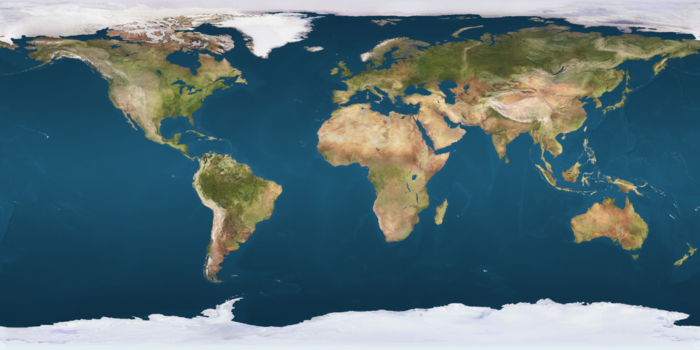
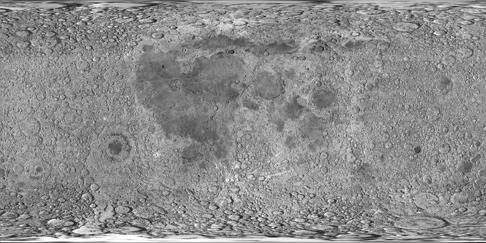
- texture
filename.png -
 load a texture map to be used for all future objects. If
filename.pngdoes not exist, instead disable texture mapping for future objects.Assume the texture is stored in sRGB and convert it to a linear color space prior to using it in rendering.
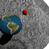
The texture coordinate used for a sphere should use latitude-longitude style coordinates. In particular, map the point at
- the maximal y to the top row of the texture image,
- the minimal y to the bottom row,
- the maximual x to the center of the image,
- the minimal x to center of the left and right edges of the image (which wraps in x),
- the maximal z to the point centered top-to-bottom and 75% to the right, and
- the minimal z to the point centered top-to-bottom and 25% to the right.
The standard math library routine
atan2is likely to help in computing these coordinates.See also Interpolate triangles for the
texcoordandtritcommands. - texture
3.5 Sampling (5–65 points)
- eye e_x e_y e_z (5 points)
-
 change the
 eyelocation used in generating rays - forward f_x f_y f_z (10 points)
-
 change the
 forwarddirection used in generating rays. Then change theupandrightvectors to be perpendicular to the newforward. Keepupas close to the originalupas possible.The usual way to make a movable vector \vec{m} perpendicular to a fixed vector \vec{f} is to find a vector perpendicualr to both (\vec{p} = \vec{f} \times \vec{m}) and then change the movable vector to be perpendicular to the fixed vector and this new vector (\vec{m}\prime = \vec{p} \times \vec{f}).
- up u_x u_y u_z (requires forward) (5 points)
-
 change the
 updirection used in generating rays. Don’t use the providedupdirectly; instead use the closest possibleupthat is perpendicular to the existingforward. Then change therightvector to be perpendicular toforwardandup. - aa n (15 points)
-
 shoot n rays per pixel (distributed
across the area of the pixel) and average them to create the pixel color
shoot n rays per pixel (distributed
across the area of the pixel) and average them to create the pixel color
- fisheye (10 points)
-
 find the ray of each pixel differently; in particular,
- divide s_x and s_y by the length of
forward, and thereafter use a normalizedforwardvector for this computation. - let r^2 = {s_x}^2 + {s_y}^2
- if r > 1 then don’t shoot any rays
- otherwise, use s_x
right, s_yup, and \sqrt{1-r^2}forward.
- divide s_x and s_y by the length of
- panorama (10 points)
-
 find the ray of each pixel differently; in particular, treat the x and y
coordinates as latitude and longitude, scaled so all latitudes and
longitudes are represented. Keep
find the ray of each pixel differently; in particular, treat the x and y
coordinates as latitude and longitude, scaled so all latitudes and
longitudes are represented. Keep forwardin the center of the screen. - dof focus lens (requires aa) (10 points)
-
 simulate depth-of-field with the given focal depth and lens radius.
Instead of the ray you would normally shoot from a given pixel, shoot a
different ray that intersects with the standard ray at distance focus but has its origin moved randomly to a
different location within lens of the
standard ray origin. Keep the ray origin within the camera plane (that
is, add multiples of the
simulate depth-of-field with the given focal depth and lens radius.
Instead of the ray you would normally shoot from a given pixel, shoot a
different ray that intersects with the standard ray at distance focus but has its origin moved randomly to a
different location within lens of the
standard ray origin. Keep the ray origin within the camera plane (that
is, add multiples of the rightandupvectors but notforward.If you do
dofandfisheyeorpanorama, you do not need to (but may) implementdoffor those alternative projections.
3.6 Speed
For real raytracers, speed is all-important: the amount of fancy things an artist can afford to do is based on how quickly the basics can be handled. These scenes are not for credit, but will give you some examples to play with if you want to try to get your code fast.
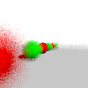
 My reference implementation can render this image in just under 1 minute
on my desktop computer or just under 4 minutes on my laptop. It makes
use of multiple suns,
My reference implementation can render this image in just under 1 minute
on my desktop computer or just under 4 minutes on my laptop. It makes
use of multiple suns, aa, dof,
shininess, roughness, and plane.
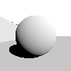
If I disable all of those, it runs in 0.2 seconds (desktop) or 0.8
seconds (laptop).
This scene is suitable for an even faster implementation because its objects are all about the same size, have little overlap, and are roughly evenly distributed across the scene, meaning more highly tuned BVH are possible.
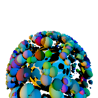
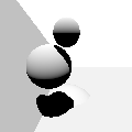
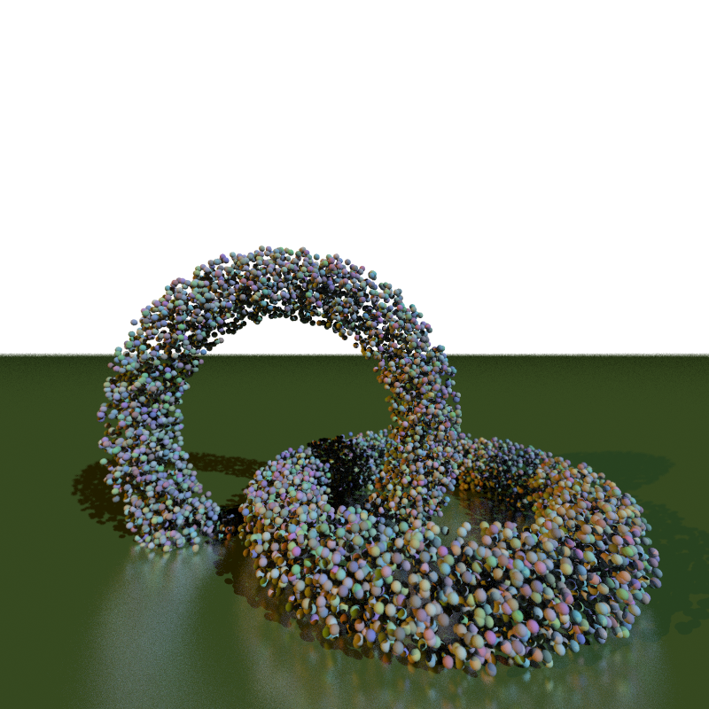
 This image has half as many spheres and half the anti-aliasing of the
previous image, but takes almost as long (50 seconds on my desktop)
because the spheres vary a lot in size and overlap a lot, which makes
acceleration more difficult.
This image has half as many spheres and half the anti-aliasing of the
previous image, but takes almost as long (50 seconds on my desktop)
because the spheres vary a lot in size and overlap a lot, which makes
acceleration more difficult.
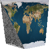
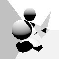
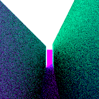
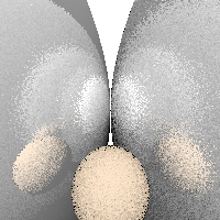
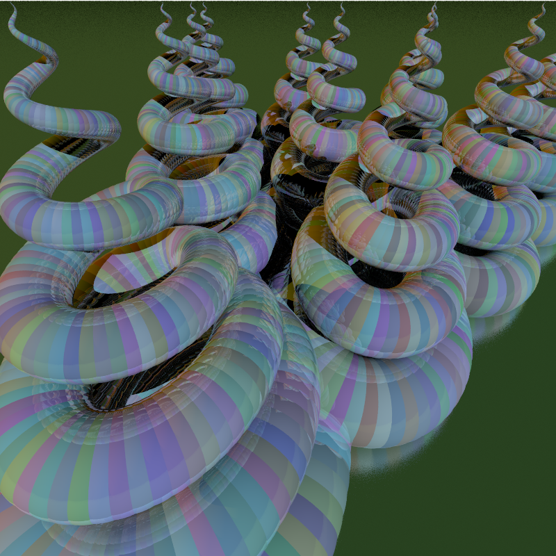
 This image has 1715 triangles, 1 plane, and 2 spheres. It uses
transparency, shininess, anti-aliasing, exposure, fisheye, and global
illumination. On my desktop my reference implementation renders it in 55
seconds.
This image has 1715 triangles, 1 plane, and 2 spheres. It uses
transparency, shininess, anti-aliasing, exposure, fisheye, and global
illumination. On my desktop my reference implementation renders it in 55
seconds.
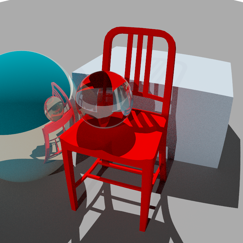
These scene also reveals some features missing from this MP, notably on the transparent sphere which lacks Fresnel-effect reflections and does not exhibit caustics: there should be a focussed spot of light in the center of that sphere’s shadow where the sphere acts as a lens fucussing the sunlight.